Source:
"In my last post, entitled Advection, I was discussing the online MODTRAN Infrared Light In The Atmosphere model.
A commenter pointed out that in the past I’d wondered about why the MODTRAN results showed that a doubling of CO2 caused a clear-sky top-of-atmosphere (TOA) decrease in upwelling longwave (LW) radiation
of less than the canonical value of 3.7 watts per square meter (W/m2) per doubling of CO2.
Here’s that data.
Figure 1. MODTRAN results for several doublings of CO2, clear-sky only, measured at the top of the atmosphere (TOA). Units are watts per square meter (W/m2).

To figure out exactly why these values were so low, I went back to the paper giving the 3.7 W/m2 value, New estimates of radiative forcing due to well-mixed greenhouse gases, by Mhyre et al.
I also recalled that in my earlier thread, commenters had mentioned that there were two “top-of-atmosphere” definitions.
One of them was what I’d used for Figure 1, looking down from 70 km above the surface.
And the other definition of “top-of-atmosphere” was the tropopause.
Upon re-reading Mhyre and doing some further research, I confirmed that the measurements and model results giving the canonical value of 3.7 W/m2 per doubling were taken, not at the actual top of the atmosphere (TOA), but at the tropopause.
The tropopause is the boundary between the troposphere and the stratosphere.
It is the location where the temperature of the atmosphere stops getting colder with altitude.
The tropopause is at different altitudes at different times and locations.
The MODTRAN model offers a graph of the atmospheric temperature profile at various locations and seasons.
Here’s the profile for what is called the “US Standard Atmosphere”.
Figure 2. Profile showing temperature versus altitude, US Standard Atmosphere

My calculations for Figure 1 were done from 70 km looking down … but as you can see, at that location the tropopause in Figure 2 is only at 11 km.
So I redid my MODTRAN runs shown in Figure 1, this time measuring from the appropriate tropopause levels at each location.
You have to take two measurements when calculating longwave changes at the tropopause—one looking upwards and one looking downwards.
The final answer is the net of the two changes.
With that as a prologue, here are my results.
I’ve compared them to the results shown in Table 1 of the Mhyre et al. paper.
My average results calculated as in the Mhyre et al. paper give a troposphere clear-sky increase in longwave (LW) absorption resulting from a doubling of CO2 of 4.97 watts per square meter (W/m2).
This is extremely close to the Mhyre et al. Table 1 figure of 5.04 W/m2 per doubling—it’s less than 0.1 W/m2 difference.
And adding in the good agreement with the CERES figures noted in my last post, these results give me confidence in the MODTRAN model.
Figure 3. As in Figure 1, except measured at the tropopause rather than from 70 km up at the top of the atmosphere (TOA).

There were a couple of surprising things about Figure 3.
First, there is a slight reduction in the change per doubling as the absolute value of the atmospheric CO2 level increases.
Unexpected.
Presumably, this reflects a gradual saturation of the absorption bands. However, it’s not large enough to affect most calculations.
Second, and more importantly, I did not expect such a large difference between measurements taken at the two levels.
The TOA measurements average about 52% smaller than the tropopause measurements.
This is interesting because of the theory of why a CO2 increase leads to surface warming.
The theory goes like this:
• The amount of atmospheric CO2 is increasing.
• This absorbs more upwelling longwave radiation, which leads to unbalanced radiation at the top of the atmosphere (TOA).
This is the TOA balance between incoming sunlight (after some of the sunlight is reflected back to space) and outgoing longwave radiation from the surface and the atmosphere.
• In order to restore the balance so that incoming radiation equals outbound radiation, the surface perforce must, has to, is required to warm up until there’s enough additional upwelling longwave to restore the balance.
I’ve pointed out the problem with this theory, which is that there are a number of other ways to restore the TOA balance.
These include:
• Increased cloud or surface reflections can reduce the amount of incoming sunlight.
• Increased absorption of sunlight by the atmospheric aerosols and clouds can lead to greater upwelling longwave.
• Increases in the number or duration of thunderstorms move additional surface heat into the troposphere, moving it above some of the greenhouse gases, and leading to increased upwelling TOA longwave.
• Increases in the amount of energy advected from the tropics to the poles increase the upwelling TOA longwave
• A change in the fraction of atmospheric radiation going upwards vs. downwards can lead to increased upwelling radiation.
So there is no requirement that surface temperatures increase in response to increasing CO2.
Increasing surface temperatures are only one among a number of ways to restore the TOA radiation balance.
With that as prologue, the insight for me from the big difference between TOA and troposphere measurements is that
I’ve been thinking that the imbalance at the actual TOA from a doubling of CO2 would be 3.7 W/m2 … but in fact, it is only about half of that, about 1.9 W/m2.
Now, as I pointed out just above, there are a variety of ways that the TOA radiation balance can be restored.
So how much of that is from surface warming?
Well, here’s the relationship between the surface temperature and the upwelling TOA longwave.
Figure 4. Scatterplot, average upwelling TOA longwave versus surface temperature, 1° latitude by 1° longitude gridcells.
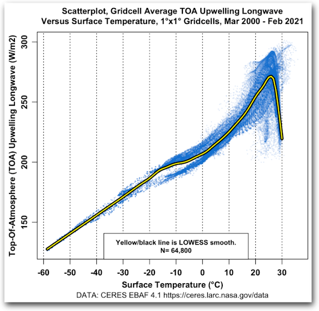
As you might expect, over much of the planet as the surface warms, the upwelling TOA longwave increases.
This makes sense, a warmer surface radiates more longwave, so you’d think there would be increasing upwelling TOA longwave.
But at temperatures above about 26°C, the situation changes rapidly.
Above that temperature, the upwelling TOA longwave drops very rapidly with increasing temperature.
I ascribe this to the action of tropical thunderstorms.
These form preferentially at temperatures above ~ 26°C.
Here’s a look at the effect using two very different datasets.
Figure 5. Rainfall from tropical thunderstorms versus sea surface temperatures.

Red dots are from the Tropical Rainfall Measuring Mission.
Blue dots are from the TAO/TRITON moored ocean buoy array.
And what is the long-term net of all of this over the entire globe?
Figure 6 shows that result.
Figure 6. Scatterplot, monthly top-of-atmosphere upwelling longwave (TOA LW) versus surface temperature.
Blue dots are from the TAO/TRITON moored ocean buoy array.
And what is the long-term net of all of this over the entire globe?
Figure 6 shows that result.
Figure 6. Scatterplot, monthly top-of-atmosphere upwelling longwave (TOA LW) versus surface temperature.

Other things being equal (which they never are), according to the CERES data a 1°C increase in global average temperature leads to a 1.9 W/m2 increase in upwelling TOA LW
… which, by what is clearly a coincidence, is the amount of the decrease in upwelling TOA LW which would result from a doubling of CO2.
It’s worth noting in this context that because we are dealing with radiation in the atmosphere, things happen at the speed of light.
A cross-correlation analysis shows that there is no delay between monthly changes in surface temperature and monthly changes in TOA longwave.
Figure 7. Cross-correlation, monthly top-of-atmosphere upwelling longwave (TOA LW) and surface temperature.

Positive values show TOA LW lagging surface temperature, negative values show surface temperature lagging TOA LW.
Overall, there is no lag between the two.
Overall, there is no lag between the two.
Since there is no lag in this, and since it directly relates surface temperature to TOA longwave radiation changes, it would seem to me that this would give a good estimate for the equilibrium climate sensitivity (ECS) of 1°C per doubling of CO2 …
Next, the calculated decrease in TOA upwelling LW ascribable to the increase in CO2 over the 21-year period is about -0.3 W/m2.
Next, the calculated decrease in TOA upwelling LW ascribable to the increase in CO2 over the 21-year period is about -0.3 W/m2.
The change in surface temperature over the period is ~ 0.4°C.
This has increased the TOA LW by ~ 0.8 W/m2 … meaning that the surface is warming more than twice as fast as would be required to offset the TOA imbalance.
This has increased the TOA LW by ~ 0.8 W/m2 … meaning that the surface is warming more than twice as fast as would be required to offset the TOA imbalance.
Why is the surface warming faster than the CO2 increase would suggest?
Well, the main reason is the increase in the amount of sunlight absorbed by the surface.
That solar energy has increased by 1.5 W/m2 over the 21-year period of the CERES record … as I said, other things are never equal.
Well, the main reason is the increase in the amount of sunlight absorbed by the surface.
That solar energy has increased by 1.5 W/m2 over the 21-year period of the CERES record … as I said, other things are never equal.
PS: In analyses such as this one, it is generally useful to keep in mind what I modestly call “Willis’s First Rule Of Climate”, which states
“In climate, everything is connected to everything else … which in turn is connected to everything else … except when it isn’t.”
“In climate, everything is connected to everything else … which in turn is connected to everything else … except when it isn’t.”
Supplemental Chart:
